Logbook

Welcome to the Pycom Logbook — a collection of news, development updates, and technical notes covering upcoming features, remote operation setup, and background on the project.

Contents

Capture Cleanup Delivers 4x Improvement in Cluster Quality #

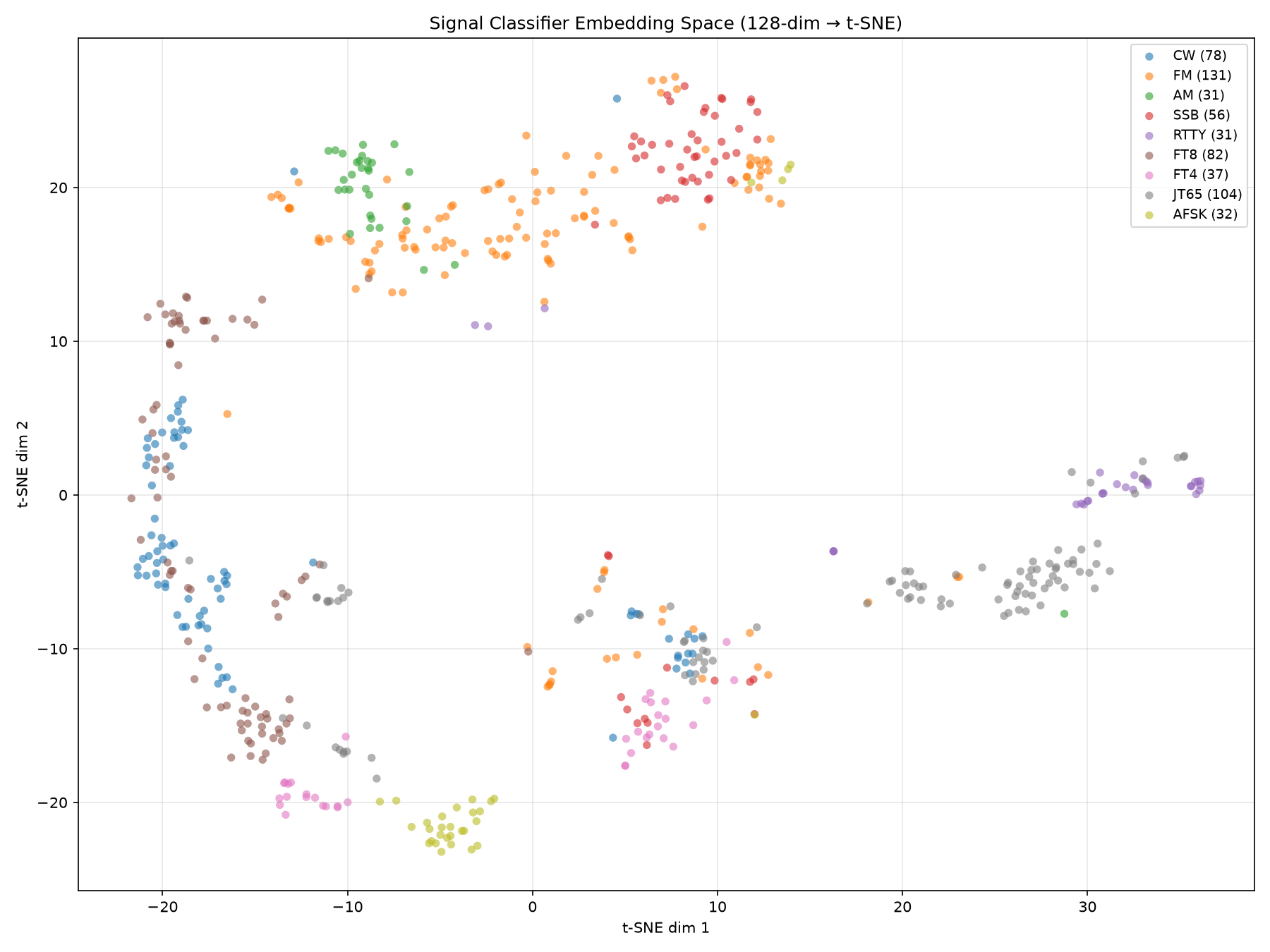
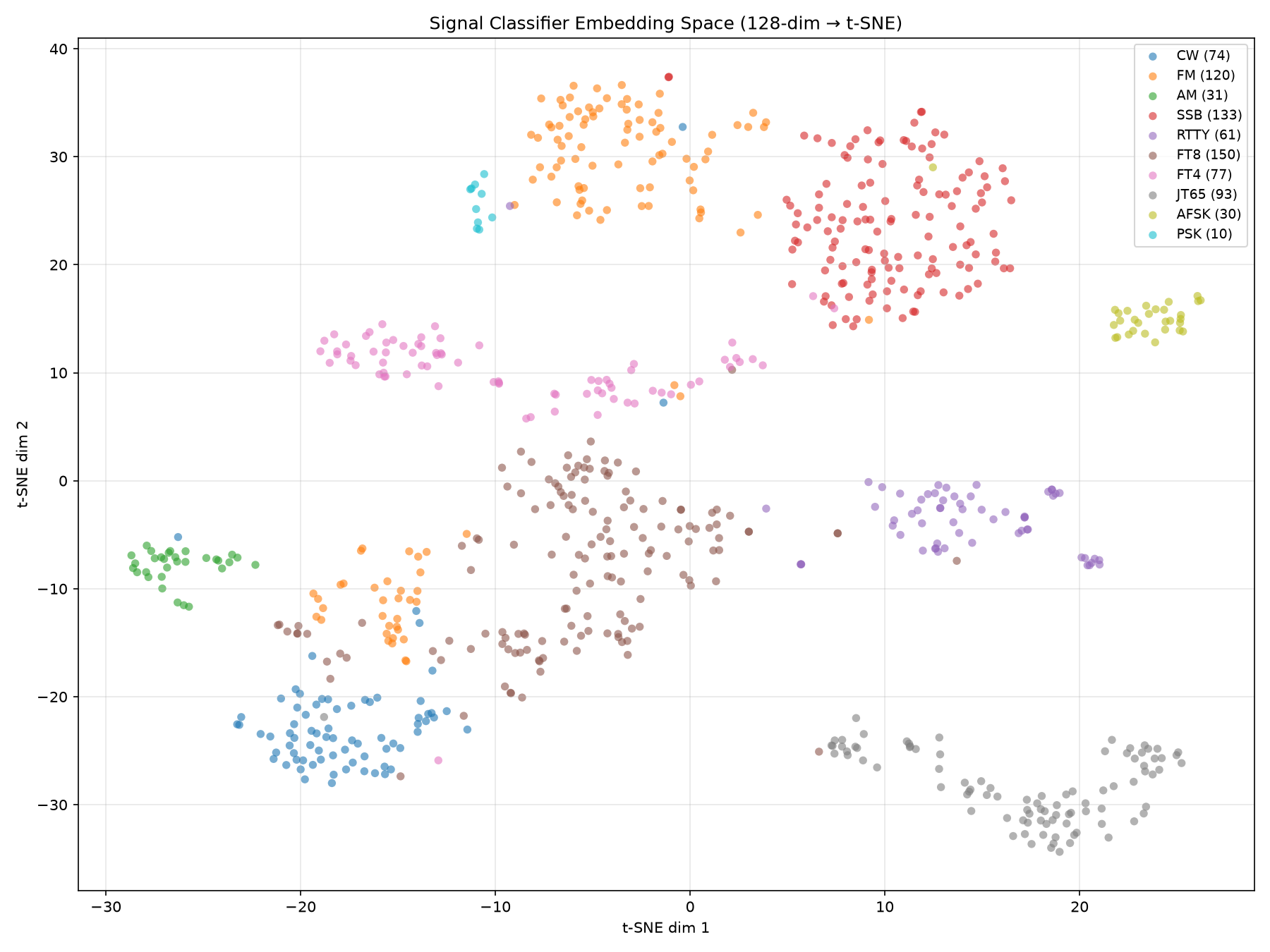
After the introspection analysis showed poor cluster separation in the t-SNE embedding, I went back through the capture dataset and cleaned up misleading captures — removing mislabelled signals, duplicates, and captures where the signal was barely visible above the noise. The improvement was immediate and significant: the silhouette score went from −0.114 (misclustered) to −0.027 (barely overlapping) — a 4× improvement. FM's intra-class spread dropped from 38.06 to 34.51, exactly as predicted in the previous post, and three FM-related confusion pairs improved substantially. The updated t-SNE projection below tells the story:

Updated t-SNE embedding visualisation after capture cleanup, showing dramatically improved cluster separation between signal classes

The overall embedding space has moved from "misclustered" to "barely overlapping," and more cleaning of the dataset should improve things further still.

Looking Inside the Classifier: Class Activation Maps and t-SNE Embeddings #

Since my last post on derived spectral features and the decision to pivot away from augmentation toward more over-the-air captures, I've been using the Verulam ARC's remote IC-9700 to generate clean, labelled signals across the missing modes. The capture count has grown from 403 to 675 training samples across 10 active classes. With the expanded dataset in hand, I wanted to understand what the model has actually learned — not just its accuracy number, but where it succeeds, where it fails, and why. Three analysis tools gave me a clear and consistent answer: Class Activation Maps (CAM) for the convolutional layers, t-SNE embedding visualisation of the 128-dimensional representation the model produces just before its classifier head, and a statistical analysis of the auxiliary feature vector.

Conv Activation Maps

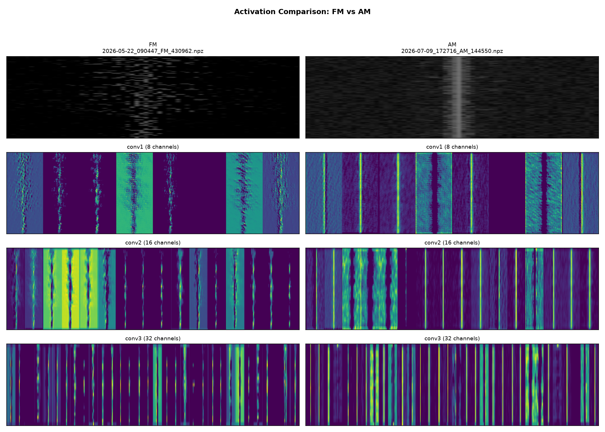
The Class Activation Map below compares which conv channels fire for FM versus AM — two modes that look very different to a human operator but can be tricky for a classifier to tell apart.

Class activation map comparing conv channel responses for FM versus AM signals

FM and AM fire largely different conv channels. AM activates the "wide signal with structure" filters — its carrier with symmetrical sidebands spreads energy across the patch. FM activates the "narrow signal" filters — the same ones CW uses, because FM's frequency-modulated carrier looks like a single spike to the CNN. The aux analysis confirms this: spectral kurtosis is the best FM-vs-AM discriminator (|d|=1.89), because AM's peaked spectrum (0.736) is very different from FM's flat-top (0.321). The separation is real, though without an ablation experiment I can't say how much comes from the pixels versus the metadata.

The key takeaway: the conv layers can distinguish FM from AM, but only through a small number of channels. Only 2 of 56 conv filters across all three layers are dead; several are discriminative, but most fire generically on both classes. The useful signal is concentrated in ch22 (AM's "wide structure" detector) and ch0/ch16 (FM's "narrow signal" detectors). This is why the model needs the aux features to get the full separation that the pixels alone can't provide.

t-SNE Embedding Space

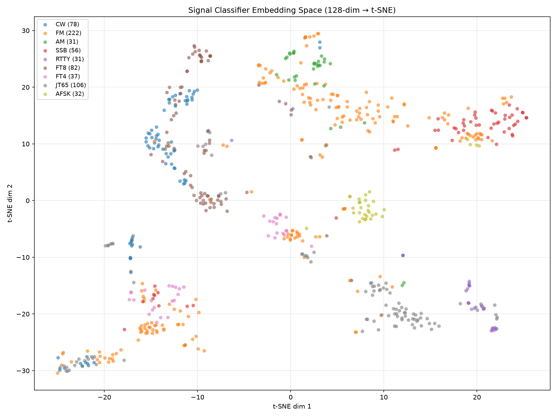
The t-SNE projection below visualises the model's 128-dimensional embedding — the internal representation it builds before the final classification layer. Each point is a training candidate, coloured by its true label. If the model had learned a clean representation, each class would form a tight, well-separated cluster. The reality is messier.

t-SNE embedding visualisation of the model's 128-dimensional representation, showing poor cluster separation between signal classes

An important caveat: this is not a pure view of the conv path. The hook captures the output after the conv features (3072-dim) and aux features (13-dim) have been concatenated and projected through a linear layer to 128 dimensions. The aux contribution is already baked in — the t-SNE is visualising the fused representation, so it can't tell us which path is doing the work.

Overall: poor cluster separation. Silhouette score = −0.114 (negative = misclustered, 0 = overlapping, 1 = perfect). The model's learned 128-dim representation does not cleanly separate the signal classes. Only 24.5 of 128 dimensions are active per sample on average (post-ReLU). 76 dimensions are completely dead — always zero across all 675 samples. 52 dimensions are ever active at all, meaning the classifier head is operating in a much smaller effective space than its architecture suggests.

RTTY is the most separated class — its centroid distance to the nearest class (JT65) is 74.3, far from all others (>90). RTTY's centroid norm (107.6) is 2–3× larger than any other class. The model strongly distinguishes RTTY's two-tone structure. At the other end, the least separated class pairs — the ones the model most confuses — are:

Least separated class pairs in t-SNE embedding space (most likely to be confused)
Class pairCentroid distance
CW ↔ FT820.1
AFSK ↔ FM27.3
FM ↔ FT427.9
CW ↔ FM29.8
AFSK ↔ FT430.2
CW ↔ FT430.6

FM ↔ AM distance = 43.3 — moderate, not close. RTTY aside, most class pairs sit between 20 and 40, which is why the overall silhouette score is negative: the clusters overlap more than they separate.

FM has the highest intra-class spread (38.06) — FM captures are scattered across the embedding space rather than forming a tight cluster. This likely reflects FM's 222 samples coming from diverse conditions: repeater vs simplex, different spans, varying SNR. The model is learning FM-specific features that vary across capture conditions rather than modulation-invariant ones. More diverse FM captures would help consolidate the cluster.

Auxiliary Feature Analysis

To complement the visual introspection, I also ran a statistical analysis of the 13 auxiliary features (the metadata the model receives alongside the image patch) to see which ones actually carry discriminative power. The table below summarises how each signal type is best differentiated from all others:

Best auxiliary feature for distinguishing each signal type
Signal typeBest featureSeparation strengthWhy
FMspan_hz1.71FM signals are genuinely wider, so operators naturally use wider spans — span_hz gives the CNN zoom-level context it needs to interpret the image patch
JT65spectral_kurtosis0.88JT65's 66-tone comb produces a very peaked spectrum
FT8center_freq_offset_hz1.39FT8 and other digital SSB modes can appear anywhere between 0 and 3 kHz — this offset reflects where signals happened to be in the passband during capture, not a modulation characteristic
CWspectral_periodicity1.73CW's on/off keying of a single carrier creates strong periodic structure in the time domain
AFSKspectral_flatness1.64AFSK is noise-like (spread energy) vs most other modes being tone-like
SSBreference_level_db0.97SSB captures were at higher ref level — partly capture practice, partly because SSB signals tend to be weaker
AMspectral_kurtosis2.07AM's carrier+sidebands produce a very peaked spectrum — the strongest single-feature separator in the whole set
RTTYspectral_flatness1.45RTTY is very tone-like (low flatness) — its two-tone structure stands out
FT4span_hz1.30FT4 captures were at narrower spans — span_hz provides zoom context the CNN needs to interpret the patch

What It All Means Together

Three tools — the class activation maps, the t-SNE embedding, and the auxiliary feature analysis — all point to the same conclusions:

  1. The conv channels show few class-specific patterns. Only 2 of 56 filters across all three conv layers are dead (3.6%), and several are discriminative — but most fire generically rather than tuning to specific signal types. The t-SNE shows that even with both image and metadata combined, the classes still don't separate cleanly.
  2. CW and FT8 are nearly impossible to distinguish at typical scope spans. All three tools agree: the conv layers see them as the same narrow spike, the t-SNE puts them closest together, and the best metadata feature (center_freq_offset_hz, |d|=1.30) separates them mainly by where the operator placed the signal, not by modulation. There is a physics-based separator — spectral periodicity also separates them (|d|=0.72, CW's on/off keying creates stronger periodicity) — but it's weak. At the spans most operators use, FT8's 8 tones are narrower than a single pixel. The model can't tell apart what it can't see.
  3. FT8 vs FT4 is the hardest pair of all. Both modes use the same 6.25 Hz tone spacing, which is narrower than one pixel at any practical scope span. Even the best metadata feature (spectral_flatness) only achieves weak separation (|d|=1.29). This pair may benefit from the temporal envelope CV feature — FT8's structured 15-second transmission cycle has a different on/off pattern to FT4's faster 4.48-second cycle, so the temporal envelope should help distinguish them where the spectral features can't.
  4. 76 of the model's 128 internal dimensions are dead. They're always zero post-ReLU, meaning their pre-ReLU values are always negative — a training artifact, not necessarily architecture waste. The average sample uses only ~25 dimensions; 52 are ever active across all samples. Shrinking the architecture from 128 to 64 would reduce parameters, but those dims might become active with more diverse data or different training. The overfitting gap (85% on training vs 66% on validation) is more likely caused by the small, imbalanced dataset (675 samples, FM=222 vs FT4=37) than by architecture size.
  5. The noise floor feature is useless. It's virtually identical across all signal types (~0.062) and contributes no discrimination at all. It's taking up a slot in the metadata vector for nothing. Removing it would tighten the model's input without losing anything.

What This Means for Next Steps

The introspection confirms the direction I set out in my previous post. The model's weaknesses are not in its architecture — they're in the data. The pixels don't contain enough information for the hardest pairs, and the metadata is carrying much of the load. The remaining work is:

  • More over-the-air captures for the under-represented modes — particularly AM, RTTY, PSK, MSK, and the other zero-sample classes. The Verulam ARC radio has been invaluable for this.
  • More diverse FM captures — different spans, SNRs, and signal conditions rather than more of the same. FM's 222 samples are the largest class but also the most scattered in the t-SNE, with the highest intra-class spread (38.06). Capturing FM at a wider range of spans and conditions would help the model learn what's consistent about FM rather than what's consistent about how I captured it.
  • Drop the dead weight. Remove noise_floor from the metadata — it's identical across all signal types and contributes nothing. This tightens the input from 13 to 12 channels.
  • Consider shrinking the model. Reducing the embedding dimension from 128 to ~64 might reduce overfitting, but it's secondary to more data and better class balance. The 76 dead dimensions are a training artifact, not necessarily waste — they might become active with more diverse data. The bigger lever for closing the train/validation gap (85% vs 66%) is likely the small, imbalanced dataset, not the architecture size.

Progress, but still work to do. The three analysis tools have given me confidence that the architecture is sound and the feature engineering is targeting the right problems — the path forward is more data and better class balance, not a fundamentally different approach.

Updated Thinking on Signal Classification: Derived Spectral Features + More Over-the-Air Captures #

My earlier post on data augmentation for Pycom's signal classifier laid out a plan to synthetically expand my small 403-sample training set with on-the-fly transforms. After more thought I realise that the plan never really sat right with me. Creating frankenstein like patches is not something I'm comfortable with, I've changed direction. Augmentation may still be on the roadmap, but it's no longer the next step — and the reason comes down to a resolution problem that augmentation can't fix.

The Resolution Problem

The IC-9700's scope produces 475 frequency bins. At the spans most operators use (5–25 kHz), each bin covers 10–53 Hz. The tone spacing of FT8 and FT4 is 80-90 Hz, and JT65's is 400 Hz — many tones of a multi-tone signal collapses into less than one bin.

ASCII waterfall visualisation showing side-by-side FT4 (left) and FT8 (right) tone patterns over 13 frames. The FT4 tones appear as faint scattered dots; FT8 tones form bright concentrated clusters (@ symbols) in these examples. Both signals occupy a narrow vertical stripe, illustrating that individual tones cannot be resolved at typical scope spans.

The 100×64 waterfall patch fed to the CNN shows a narrow vertical stripe with no resolvable tone structure at all. No amount of amplitude scaling, noise injection, or frequency shifting will conjure detail that isn't in the pixels to begin with. Augmentation diversifies the views of information the model already has; it doesn't add the information the model is missing.

Given my small sample data set and obfuscation of the signal captured over the air:

  • Information the CNN can't extract → solved by derived spectral features: seven statistical descriptors computed from the 100-frame scope history that capture modulation characteristics invisible in the image patch.
  • Classes the model has never seen → solved by more over-the-air captures: eight of Pycom's fifteen supported modes have zero training samples, and the remaining seven are badly imbalanced (FM 160, SSB 9). No feature engineering fixes a class the model has never been shown.

Seven Derived Spectral Features

The auxiliary feature vector fed to the classifier alongside the image patch has grown from 6 channels (span, reference level, noise floor, bandwidth, frequency offset, SNR) to 13. The seven new descriptors are computed from the signal's averaged spectrum and temporal envelope in under a millisecond per candidate. Each one captures a different aspect of spectral shape that the CNN patch cannot resolve at typical scope spans:

Seven derived spectral features for signal classification
#FeatureWhat it measuresHow it helps differentiate signal types
1Spectral Flatness (Wiener Entropy)Whether the signal is "tone-like" (all power at one frequency) or "noise-like" (power spread evenly). Ratio of the geometric mean to the arithmetic mean of the power spectrum — a standard measure from speech and audio analysis.Pure-tone CW sits near 0; broad/noise-like modes like FT4 (~0.06) and AFSK (~0.03) sit higher. Best single separator for FT4 vs CW (3.1σ) and JT65 vs FT4 (3.0σ).
2Spectral KurtosisHow "spiky" the amplitude distribution is — the 4th standardised moment, measuring peakedness and tail weight. A single sharp carrier produces high kurtosis; a flat or multi-peaked spectrum produces low or negative kurtosis.JT65's 66-tone comb structure produces extreme kurtosis (~10.4) while FT8's flatter distribution is actually negative (-0.6). Resolves confusion pairs that flatness can't — e.g. AFSK vs FT8 (2.1σ).
3Peak CountThe number of distinct amplitude peaks above the noise floor + 3 dB in the averaged spectrum. CW is one peak, RTTY is two, FSK is several.Perfectly separates FT4 from CW, and cleanly distinguishes single-tone (CW=1) from multi-tone (FSK~4+) modes even when individual tones aren't resolvable.
4Spectral PeriodicityThe strength of comb-like structure in the spectrum — found by taking the FFT of the magnitude spectrum and measuring the dominant periodic component. Multi-tone MFSK signals produce evenly-spaced peaks even when the tones themselves blur together.The star performer: achieves >3σ separation on four confusion pairs. AFSK vs FT8 (7.8σ), CW vs FM (7.1σ), CW vs SSB (5.4σ), FT8 vs JT65 (3.7σ). Detects MFSK comb structure that's invisible in the image patch.
5Spectral Bandwidth RatioHow spread out the spectral energy is around its centre of mass, normalised by the signal region width. A narrow CW spike has low bandwidth ratio; a wide FM signal has high.Strongest single separator in the whole set: FT4 vs CW at 8.6σ. Distinguishes narrow signals (CW, FT4) from wide ones (FM, SSB) more discriminatively than the raw occupied bandwidth.
6Centroid OffsetHow far the spectral centre-of-mass sits from the geometric centre of the signal region — a measure of spectral asymmetry. A symmetric signal (FM with equal sidebands) centres near 0; a one-sided signal (SSB) is offset.Separates FM's symmetric sidebands from SSB's one-sided energy, and distinguishes centred modes like AFSK (0.01) from slightly-offset modes like FT8 (0.08) at 2.8σ.
7Temporal Envelope CVFrame-to-frame energy variation across the 100-frame scope history — the coefficient of variation of total energy per frame. Bursty signals vary a lot; continuous carriers vary little.CW's Morse on/off keying is bursty (high CV); FM and PSK carriers are continuous (low CV). Distinguishes on/off-keyed modes from continuous modes in a way no single-frame feature can.

Taken together, the seven features improve 9 of the 10 measured confusion pairs (signals that the model otherwise confuses eg; FT8/FT4). The one holdout is FT8 vs FT4 — both use 6.25 Hz tone spacing and collapse to the same sub-pixel width at every span above 2.5 kHz. The only real difference is occupied bandwidth (FT8: 80 Hz, FT4: 90 Hz), which is weakly captured.

More Over-the-Air Captures

The remaining weakness isn't an architecture problem — it's a data problem. Eight of fifteen supported modes (AM, RTTY, FT2, Q65, PSK, FSK, MFSK, MSK) have zero training samples, and the seven that do exist are heavily skewed toward FM and JT65. No feature, however well-engineered, teaches a classifier a class it has never been shown. The fix is to generate more labelled over-the-air captures, particularly for the under-represented modes.

To that end I have reached out to the Verulam Amateur Radio Club who have kindly agreed that I can use the remote Icom 9700 — so I can transmit clean, labelled examples of AM, RTTY, PSK, MSK and the other missing modes and capture them directly through the IC-9700's scope, without having to endure the cost of purchasing a second radio. This gives data without relying on whatever happens to be on the bands, and lets me balance the class distribution deliberately rather than opportunistically. The earlier O'Shea et al. (2018) finding still stands — models trained on clean data degrade over the air — so once the class-coverage gap is closed with real captures, the augmentation transforms from the previous post (noise injection, frequency shifting, Mixup) may come back to harden the model against the SNR, carrier-offset, and multipath variation it'll meet at inference time.

Pycom Radio Controller Demo and Live RS-44 Contact #

AMSAT Satellite Status Reports #

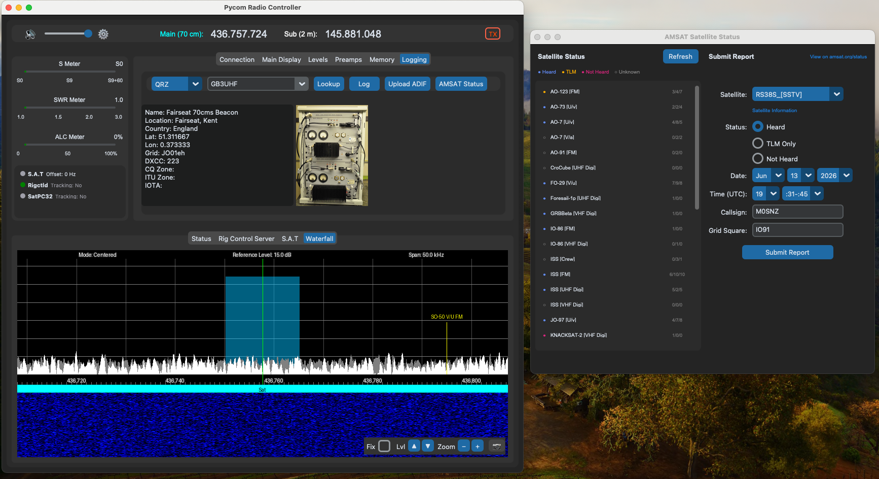
It's about time. Pycom's next release will allow you to submit satellite status reports directly to AMSAT — no need to switch to a browser to log that you heard (or didn't hear) a satellite. The new AMSAT Status dialog shows current satellite status at a glance, auto-fills your callsign, grid square, time and the tracked satellite from S.A.T (if in use), and submits reports with a single click.

AMSAT satellite status report dialog showing satellite list and submission form

Thinking about Training Data Augmentation for Signal Classification #

Two influential papers in Automatic Modulation Recognition (AMR) provide clear guidance for improving Pycom's signal classifier. O'Shea, Roy & Clancy's Over-the-Air Deep Learning Based Radio Signal Classification (IEEE JSTSP, 2018) demonstrates that models trained only on clean, ideal data degrade dramatically when deployed over the air, where carrier frequency offset, varying SNR, and multipath effects conspire to confuse the classifier. Li, Wang, Dong & Wang's Data Augmentation for Automatic Modulation Recognition (IEEE Wireless Communications Letters, 2025) shows that targeted augmentation — particularly noise injection, channel impairment simulation, and synthetic data generation — significantly improves classification accuracy, especially for underrepresented signal types at low SNR.

Pycom's architecture already mitigates the worst of the over-the-air pitfalls: the center_freq_offset_hz auxiliary feature directly encodes the carrier offset that was identified as the primary error source, and the six-channel auxiliary input (span, reference level, noise floor, bandwidth, frequency offset, SNR) gives the model explicit metadata about signal conditions rather than forcing it to infer everything from pixels. Bandwidth-aware centred patch extraction normalises the view regardless of mode width, and WeightedRandomSampler balances class representation during training. What both papers make clear is that architectural design alone isn't enough — the model also needs to see the full range of variation it will encounter at inference time, and that's where augmentation fills the gap.

The current ScopeCNN-Patch (Convolutional Neural Network) model was trained on just 403 samples across seven active signal classes — FM (160), JT65 (95), CW (73), FT8 (35), FT4 (17), AFSK (14), and SSB (9) — achieving 77% validation accuracy. Eight of the fifteen supported modes have zero training data. This severe class imbalance means the model can recognise strong FM and CW signals reliably but struggles with underrepresented modes like SSB and FT4, where it simply hasn't seen enough variation to generalise. The augmentation approach directly addresses this: rather than requiring hundreds more captures (which means more time at the radio, and potentially investing in something like an IC-7100 so I can generate my own signals to capture), we can apply five on-the-fly transforms during training that synthetically expand each sample into many unique training views. The model sees different augmented versions of the same signal every epoch, teaching it that the same mode can look different under varying conditions.

Augmentation transforms applied during classifier training
TransformWhat It SimulatesWhy It Matters
Amplitude scalingRF gain and AGC variation (70–120% intensity)Most basic real-world variation — no two contacts have the same signal strength
Additive noise (SNR-aware)Poorer SNR conditionsHighest-impact technique per the literature. Scales noise proportionally to each patch's existing floor, preserving the character of quiet and noisy signals alike
Frequency shiftingImprecise centre-frequency tuningSlides the signal left or right by a few bins; directly complements the center_freq_offset_hz auxiliary feature
Time shiftingPartially-filled scope display after tuningDrops rows from the top and zero-fills the bottom, simulating the display right after changing frequency
Auxiliary feature jitterVariation in measured metadataPerturbs noise floor, frequency offset, and SNR channels slightly; prevents memorisation of exact values for rare classes
Same-class MixupAdditional within-class variationBlends two patches of the same signal type at random ratios for classes with fewer than 20 samples, creating plausible new views without label noise

Augmentation would be enabled by default for training from scratch and disabled for fine-tuning to preserve the feature distribution the frozen layers expect. The expected improvement is from 77% to 80–85% overall, with the biggest gains on minority classes like SSB and AFSK.

IARU Band Plan Display #

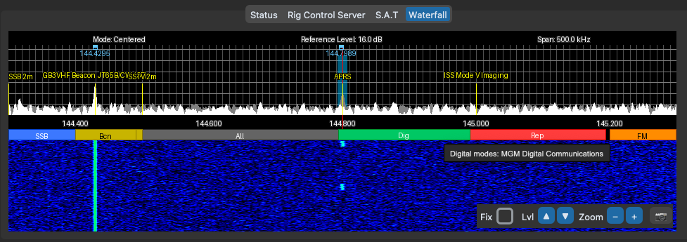
The waterfall now includes a colour-coded band plan strip showing IARU allocations for your region. Hover any segment to see its category and description — no more guessing which part of the band is reserved for CW, where the satellite sub-band starts, or whether that frequency is in the FT8 window.

Band plan strip on waterfall showing IARU region allocations

Multi-Region Support

Band plans differ across the three IARU regions. Pycom ships with allocations for all three, sourced from RSGB (Region 1), ARRL (Region 2), and the IARU Region 3 interim band plan. Select your region in Configuration → General → IARU Region and the display updates immediately — no restart needed.

IARU band plan regions and their sources
RegionCoversSource
Region 1Europe, Africa, Middle East, Northern AsiaRSGB
Region 2AmericasARRL
Region 3South Asia, East Asia, OceaniaIARU Region 3

Categories

The band plan strip uses 15 colour-coded categories so you can identify segments at a glance:

CW, All modes, WSPR, FT8, FT4, FM, Repeaters, Beacons, Satellite, EME, Digital modes, SSB, ATV, APRS, and DX. Shared calling frequencies (like FT8 at 144.174 MHz) appear in all regions regardless of your selection.

Customising the Band Plan

The band plan data is stored in bandplan.csv in your Pycom configuration directory (~/Pycom/ on macOS, %USERPROFILE%\Pycom\ on Windows). The file is modifiable — edit it to add, remove, or change allocations to match your local band plan. Pycom will replace it with the default on start-up only if the file doesn't exist; your changes are never overwritten.

Full 70cm Coverage for Region 2

Region 2's 70cm allocation spans 420–450 MHz, wider than Regions 1 and 3 (430–440 MHz). The band plan strip and frequency labels cover the full range, so Region 2 operators see their complete allocation on the waterfall.

Pycom Development #

Pycom has evolved from a repository where every line of code was written manually to a fully agentic development stack. Using opencode — a CLI-based AI coding environment — backed by the Ollama Pro plan with access to the GLM-5.1 Cloud model (currently around £15/month), the project now operates with custom skills, specialised agents, structured expertise management, and automated quality gates that keep the codebase consistent and the protocol layer correct. The combination of opencode's skill system and a capable cloud-hosted model means every session starts with deep project context and ends with consistent, reviewed and tested code.
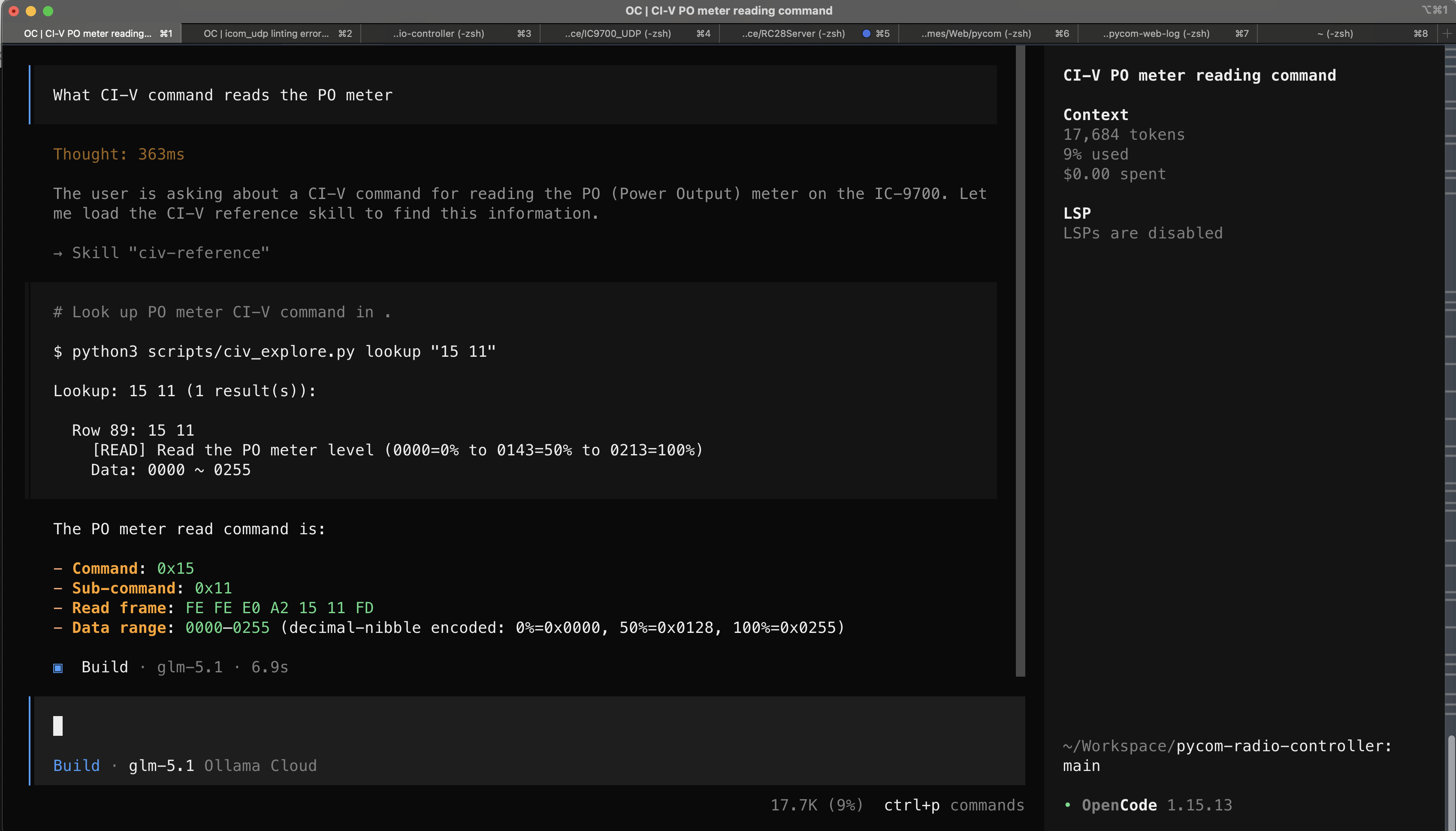
Opencode development screenshot

From Solo to Agentic

In the early days, every feature, bug fix, and protocol implementation was hand-coded and tested against the radio. The codebase has grown to over 25,000 lines across 40+ modules, with a CI-V command reference spanning 542 commands. Managing that complexity manually was becoming unsustainable. Today, opencode is configured with persistent context — AGENTS.md, docs/CODING_STANDARDS.md, and docs/PR_REVIEW_CRITERIA.md — that guides every session. These files encode project conventions (decimal-nibble encoding rules, threading constraints, naming standards, read-only library boundaries) so that the AI agent produces code that is consistent with the existing codebase from the start, rather than needing correction afterwards.

A dedicated expertise manager called mulch records patterns, failures, decisions, and conventions across sessions. Before each task, opencode queries mulch to avoid re-introducing known-bad patterns or repeating investigations that were already resolved. Findings are recorded under domains like gotchas, architecture, connection-flow, and scope-protocol, building a living knowledge base that persists between conversations.

Custom Skills & Tools

opencode skills provide domain-specific expertise on demand. Each skill is loaded contextually — when a question or task matches its domain, the full skill instructions and reference data are injected into the session. The table below shows the skills currently configured for Pycom:

opencode skills configured for the Pycom project
SkillPurposeMechanism
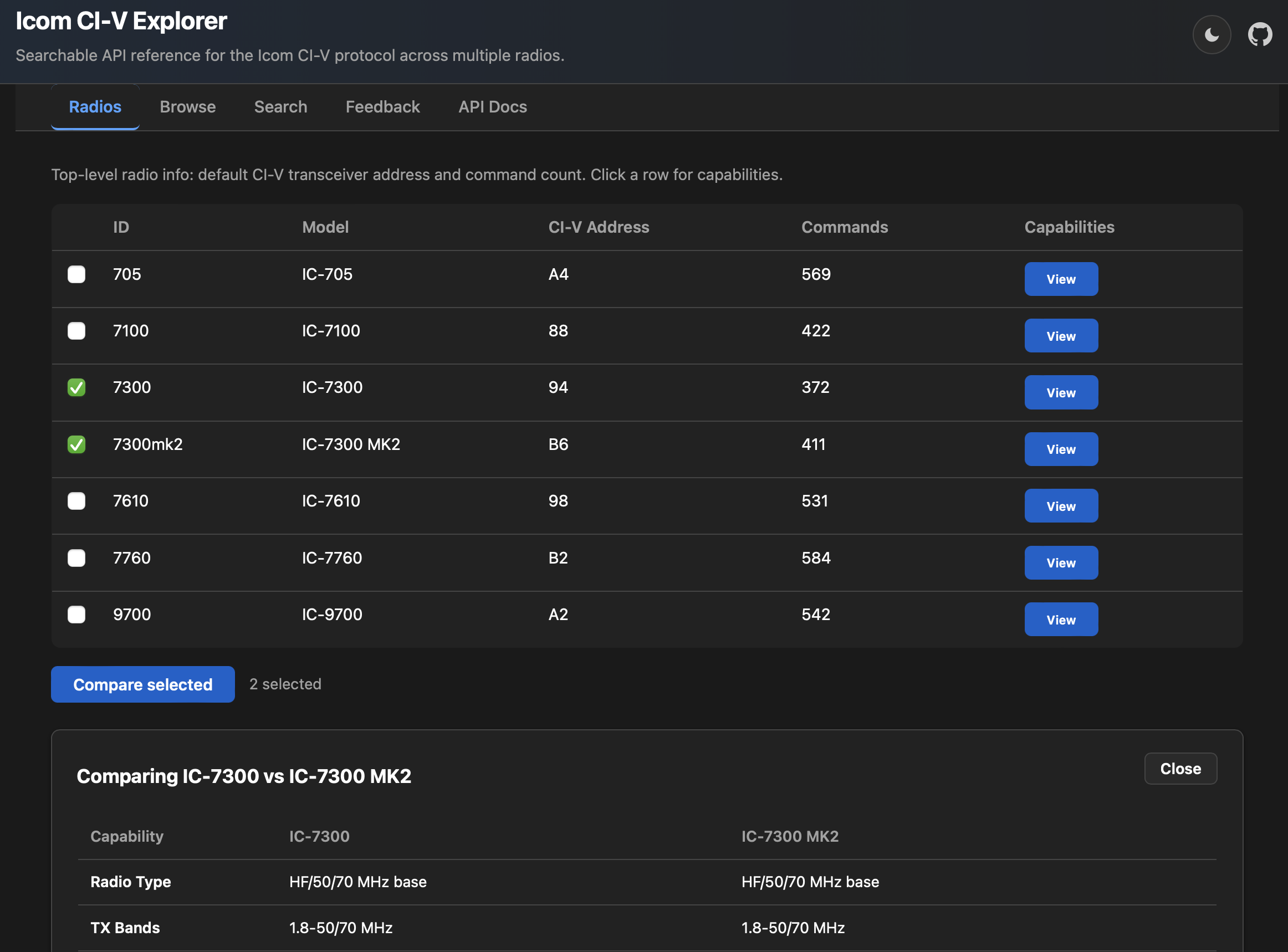
CI-V ReferenceLook up IC-9700 CI-V commands, hex codes, data encodings, sub-commands, and protocol detailsscripts/civ_explore.py — parses the 542-command reference CSV and auxiliary encoding docs. Subcommands: search, lookup, info, encoding, frame, validate
Pcap DebuggerAnalyse ICOM 9700/7610 Wireshark network traces — decode control, CI-V, and audio streams; inspect socket lifecycle and protocol compliancepcap_explorer.py — dissects pcap/pcapng files, extracts CI-V command/response pairs, audio streams, and timing data
Signal Model SyncSynchronise, retrain, and verify the ONNX signal classifier between the project and ~/Pycom/signals/scripts/sync_signals_dir.sh — runs verification, fine-tuning, and model deployment in one step
Model RetrainingRetrain the ONNX signal classifier from labelled captures and deploy to distscripts/retrain_model.py — supports --fine-tune from bundled base model and --from-scratch modes
Expertise ManagementRecord and query structured project expertise across sessionsmulch CLI (v0.6.3) — domains: gotchas, architecture, connection-flow, scope-protocol, op-log-level, python-style, test-automation
Test RunnerDiscover, run, and diagnose tests with full pytest/coverage integrationpytest with SerialMock, flake8 lint classes, venv isolation via scripts/run_tests.sh
Persistent ContextGuide every session with project conventions, constraints, and coding standardsAGENTS.md, docs/CODING_STANDARDS.md, docs/PR_REVIEW_CRITERIA.md — loaded automatically by opencode at session start

Specialised Agents

Beyond skills, opencode is configured with dedicated subagents that handle specific workflows autonomously:

  • PR Reviewer — Analyses pull requests and diffs against project standards (coding conventions, threading rules, CI-V protocol constraints, read-only boundaries). Catches architectural violations before merge.
  • Docs Maintainer — Audits documentation for staleness, duplication, and inconsistency. When features change, it updates the relevant docs to stay in sync with the code.
  • Test Runner — Discovers and runs the appropriate test modules, interprets failures, and suggests fixes. Knows the project's pytest configuration, coverage targets, and SerialMock patterns.
  • Explore Agent — Fast codebase search for files, patterns, and architectural answers. Used when you need to find "where is X implemented" or "how does Y work" without reading every file.

Two Repositories

Pycom's codebase is split across two repositories:

  • pycom-radio-controller — The main application repository. Contains the GUI, radio controller, signal detection, satellite tracking, configuration, and all the agentic tooling described above.
  • ICOM_UDP — A separate repository containing the ICOM UDP transport library. This provides scope data parsing, audio streaming, and network-based CI-V communication for radios with built-in Wi-Fi/Ethernet.

The UDP library is copied into the main repo at lib/icom_udp/ as a read-only dependency. Files are set chmod 444 to prevent accidental edits. All changes must be made upstream in the ICOM_UDP repository first, then synced via scripts/sync_icom_udp.sh. This separation ensures the library can be developed and tested independently while keeping the main repo's copy in sync.

Self-Hosted Gitea

All source control, CI, and issue tracking runs on a self-hosted Gitea instance. The setup provides:

  • Git hosting — Private repositories for both pycom-radio-controller and ICOM_UDP, with full branch and merge management.
  • CI Action Runner — A Gitea Actions workflow (.gitea/workflows/pyinstaller.yaml) builds distributable packages on every push to main. It produces a macOS .app bundle and a Windows .exe, both packaged for distribution. The build excludes dev-only dependencies (pytest, coverage, flake8, torch) via --exclude-module flags.
  • Issue tracking — Bugs, feature requests, and milestone tracking (including the UDP transport migration plan) are all managed in Gitea Issues.

Test Suite

The Pycom test suite is built on pytest with hardware-free testing as a core principle. Since the app communicates with a physical ICOM IC-9700 via serial, every test must work without the radio connected:

Pycom test suite categories and approach
CategoryFilesApproach
Protocol & Encodingtests/radio/test_pycomIC9700.pyPure-function tests for BCD, decimal-nibble, and CI-V frame construction — the highest-value tests in the codebase
Radio Controllertests/radio/test_radioController.pyThreaded command queue with SerialMock — verifies queue semantics, timeout handling, and factory creation
Signal Detectiontests/signal/ (4 files)Statistical detector, classifier, patch extraction, training metadata
Satellite Trackingtests/csnsat/test_csnSatManager.pyDoppler rate calculation, offset handling, polling logic with mocked network calls
Config & Providerstests/config/, tests/provider/Config round-trips with temp directories, API response parsing with mocked requests
Rigctl & RC-28tests/rigctl/, tests/rc28/TCP command parsing, HID event parsing — no hardware needed
Build & Linttests/build/test_syntax.pyast.parse syntax validation + flake8 critical/lint checks integrated as pytest classes
Regressiontests/regression/test_known_bugs.pyKnown bugs documented as tests — fail until fixed, then become permanent guards

Every test run creates a fresh virtual environment via scripts/run_tests.sh, installs dependencies, runs the full suite with coverage, and tears down — ensuring no contamination between runs. Coverage targets range from 90%+ for protocol/encoding code down to 40% for GUI code, with an overall target of 75%+.

The Agentic Advantage

The transition from solo manual coding to agentic development has fundamentally changed the pace and quality of Pycom's delivery. In the months since adopting the opencode stack, features that previously took weeks of careful manual implementation — each requiring protocol reference lookups, encoding verification, threading audit, and manual testing against the radio — now ship in days or even hours. The CI-V Explore skill eliminated constant context-switching to the ICOM manual; the pcap debugger turned hours of trace analysis into minutes; mulch ensures that hard-won knowledge about decimal-nibble gotchas and threading constraints is never lost between sessions.

Recent feature velocity illustrates the shift: AI signal detection and classification with a trainable ONNX model and 15-mode classifier, 542-command CI-V coverage with validated encoding reference, full UDP transport library integration for network-based radio control, and a redesign of the main display tab with enhanced support for dual transceivers — all developed and merged with AI-assisted code review, automated testing, and structured expertise management. The test suite alone grew from zero to 45+ test files covering protocol encoding, command queues, signal processing, configuration, and regression guards — something that would have taken far longer to build manually.

The key insight: agentic development doesn't replace understanding — it amplifies it. The project's AGENTS.md, coding standards, and mulch expertise records ensure the AI operates within well-defined constraints, while the specialised agents handle review, documentation, and testing that would otherwise be bottlenecks. The result is a system that allows me to test ideas and ship faster without cutting corners.
Automatic Signal Detection & AI Identification #

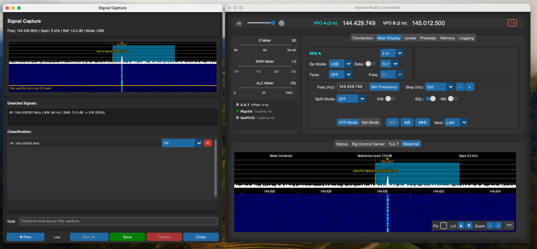
Pycom can automatically detect signals on the waterfall and classify them using a built-in AI model — no manual scanning required. Configure sensitivity with three presets or eight tuneable parameters, capture signals for review, and train your own model from real off-the-air data. See the Signal Detection, AI Identification, and Signal Reference pages for full details.

Signal capture and classification

Signal Detection

The statistical detector runs in real time alongside the waterfall, finding signal groups that stand out from the noise floor. Choose from Normal, Sensitive, and Strong Only presets, or adjust individual parameters like detection percentile, and minimum contrast Z to suit your operating conditions. Detection is automatically suppressed during transmit to prevent overloading the detector.

Signal Capture & Labelling

Detected signals appear in the capture window sorted by frequency. Select any candidate or drag select a section on the waterfall to inspect a specific signal, then assign a label from the 15 supported signal types — or mark it as Unknown. Add notes, adjust the label, and capture as many examples as you need to build a training dataset.

AI Classification

The built-in ONNX neural network classifies detected signals against 15 mode types including CW, FM, FT8, JT65, SSB, and more. A confidence threshold (default 50%) filters out uncertain predictions. The distributed model achieves 77% validation accuracy on signals with training data at present, and you can reload a fine-tuned model without restarting the app. As I capture more signals, they will be automatically added to new distributions of the application. Contact me on Discord and share your classified signals for them to be included in the application.

Train Your Own Model

Collect captures, label them, and retrain the classifier to recognise the signals you encounter on your own bands. Use python retrain_model.py --fine-tune to add your data to the distributed base model, preserving what it already knows while learning new patterns. Or train from scratch for full control. Quality warnings alert you to class coverage gaps, data imbalance, and accuracy regression before the new model is deployed.

CI-V Command Executor #

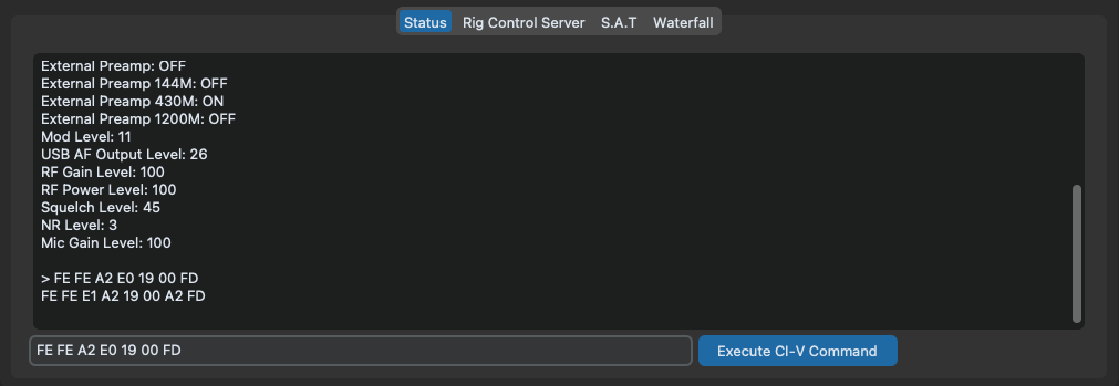
The Status tab includes a CI-V command executor for sending raw commands directly to your IC-9700. This is useful for experimenting with commands that aren't exposed in the GUI, reading radio state, or diagnosing communication issues.

Execute CI-V commands directly from the UI

How It Works

The command field is pre-filled with the CI-V preamble and addresses (FE FE A2 E0 in my case). Enter your command and data bytes after the preamble, add a terminating FD, then click Execute CI-V Command. The radio's response (or an error message) appears in the status text area above.

Examples

CI-V command examples for the IC-9700
CommandDescriptionResponse
19 00Read transceiver IDReturns the transceiver ID for IC-9700
03Read operating frequencyBCD-encoded, e.g. 00 00 00 44 01 = 144.000 MHz
04Read operating modeMode byte + filter bandwidth
1C 00Read TX/RX status00 = RX, 01 = TX
15 02Read S-meter levelDecimal-nibble percentage (0–255)
14 0ARead RF power levelDecimal-nibble percentage (0–255)
14 03Read squelch levelDecimal-nibble percentage (0–255)
16 5ARead satellite mode status00 = OFF, 01 = ON

The full CI-V command reference contains over 540 commands refer to the ICOM IC-9700 instruction manual for complete details on data encoding.

UDP Transport Library — Preview #

The UDP transport library has now been fully integrated into Pycom. Network connectivity is available in the latest release — see the download page.

The video below shows a fully implemented library that I've created for using the radios built in Wi-Fi/ethernet server over the network. I'm currently working on integrating this with Pycom so that it's no longer tied to a USB connection. Benefits include integrated audio and faster responsiveness including scope.

Measure Base Station performance using S.A.T and FT4 Satellite Loopback #

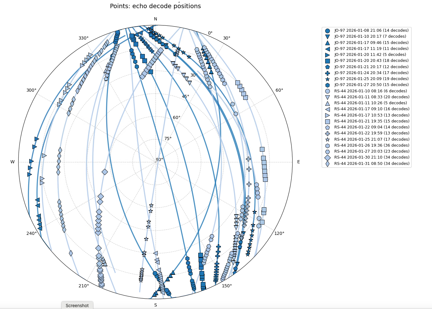
Pycom can log every S.A.T update to with precision, along with WSJTX log files it's possible to create polar plots for multiple satellite passes from your base station. At the default one-second polling interval, each entry captures the satellite's position, applied doppler, and the exact frequencies in use at that moment:

2026-01-30 21:09 INFO [Pycom.lib.csnsat.csnSatManager] Timestamp: 21:09:40, Sat: RS-44, Az: 202.978245, El: -0.136604, Range km: 4338.595298, Main: 435620549, Sub: 145990135, Doppler up: -2865, Doppler down: 8549, Doppler up rate: 0, Doppler down rate: 0, Offset: 0, Tracking: Reverse, Freq Scaling: OFF, RIT: OFF, RIT Freq: 0

Dual WSJT-X Instances

Two instances of WSJT-X run simultaneously — one to generate and transmit FT4, the other to receive and decode the repeated signal. This is set up by duplicating the WSJT-X shortcut, renaming it (e.g. wsjtx - RX), and appending --rig-name=None to the target. Each instance maintains its own log directory, accessible from the file menu.

WSJT-X communication logs are stored in ALL.txt and contain precise timing, frequency, mode, SNR, and offset for each decoded message:

            260123_102722   435.118 Rx FT4     -1  0.3 1081 CQ DL3NGN JN59
            260123_102730   435.118 Tx FT4      0  0.0 2245 CQ M0SNZ IO91
            

Post-Pass Analysis

Scripts for post-pass processing and creating polar plots of satellite passes are available at github.com/stevendodd/Sat-Analysis.

Multi pass polar plot

USB Remote Operation #

Pycom now fully supports network connectivity and is no longer tied to USB. See the radio setup guide for network connection details.

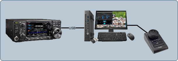
Initial Local Installation

Local installation diagram

Of course you can use the software locally where you install and operate the software on your shack computer.

Audio is available via the USB serial connection. Speakers and microphone connected to the radio should be automatically installed on your operating system when you install the USB drivers.

There is support within Pycom for a local RC-28 controller and you can run doppler tracking or other software on the same computer; however the software comes into its own when you want to start to operate remotely.

Remote Setup

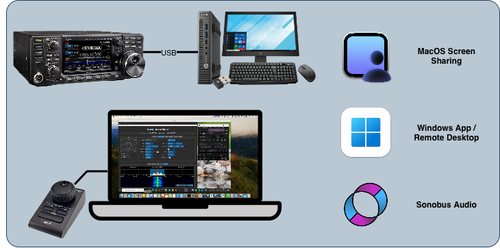
Once you have the software installed on your shack computer, you can use tools such as Microsoft Windows App or MacOS Screen Sharing to view the display and control the computer remotely. Audio can be streamed over the network both to and from the shack computer using tools like Sonobus. There is also support for a remotely connected RC-28 controller. Using a combination of these tools (or alternatives if you prefer) you can have full operational capabilities when you're away from your shack.

Remote installation diagram

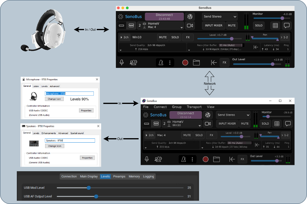
Remote Audio Chain

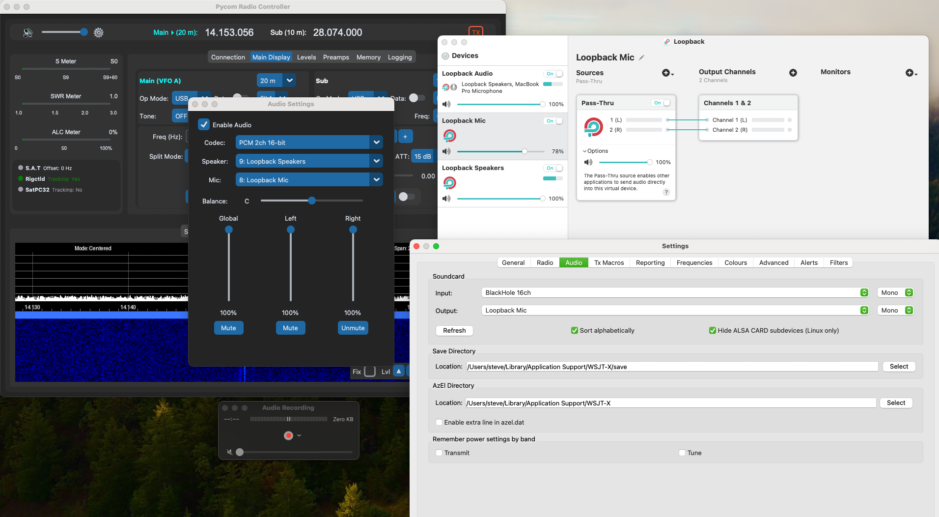
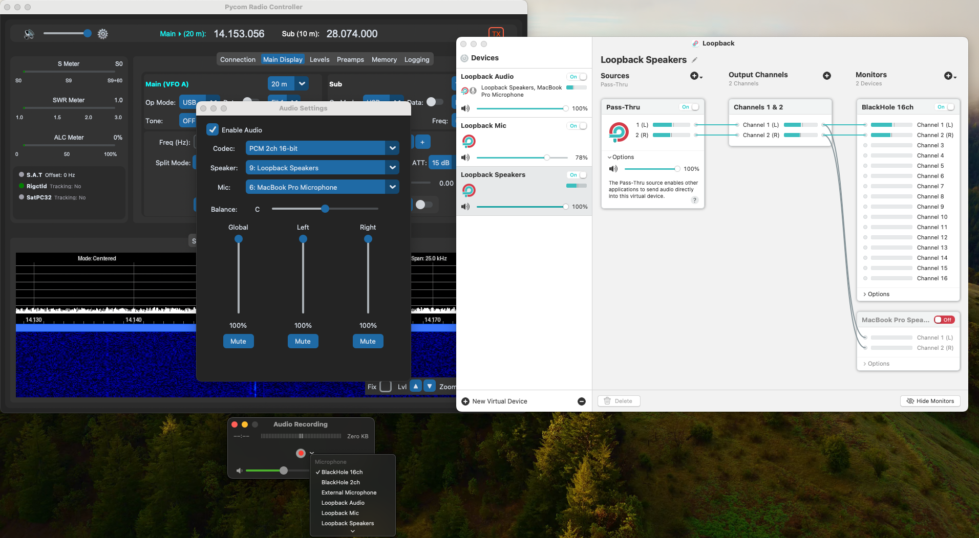
Connecting remote audio involves configuring levels at each component in the chain, including within the Pycom software. In addition to the components documented in the diagram I also pass audio out of the local SonoBus to Blackhole Audio which allows me to record audio for playback later. I have a wired ethernet network between the two computers however it is possible to reduce the audio quality without too much impact for streaming over the Internet.

Remote audio chain diagram

Development Environment My Specific Configuration #

Development environment hardware and software configuration
Component Detail
Shack Computer HP EliteDesk 800 G3 Small Form Factor Business PC
4 x Intel(R) Core(TM) i5-7600 CPU @ 3.50GHz (1 Socket)
46 GB DDR4 RAM
Proxmox Virtual Environment 8.4.1
Operating systems Window 10 virtual machine with 2 virtual CPUs and 16GB RAM
macOS Monterey (Intel) virtual machine with 2 virtual CPUs and 4GB RAM
macOS Sonoma (Silicon) Apple M1 with 16GB RAM
USB Drivers Icom USB Drivers installed. For MacOS I used CP210x VCP Mac OSX Driver
Remote control software Windows App
macOS Screen Sharing
Sonobus
RC-28 Server
Doppler tracking CSN Technologies S.A.T (preference)
Gpredict
SatPC32
Antenna rotation PstRotator
Gpredict
Both underpinned by my own custom rotctld implementation

Making Amateur Radio Accessible #

Although there are many reasons why you might want remote control, the motivation for creating this software was a desire to operate satellites specifically linear satellite and finding a lack of support from currently existing software on the market.

In 2018 I had a surfing accident and was pulled out of the sea by a lifeguard from RNLI. I was left paralysed with a spinal cord injury from the neck downwards. I've recovered sufficiently to be able to use a trackpad awkwardly with the middle finger on my left hand however turning dials and pushing buttons on a radio is a little bit beyond me. Using Pycom Radio Controller remotely allows me to operate successfully without limitations.

You can find out more about the origins of the software and Making Amateur Radio Accessible on the RSGB Tonight@8 episode and information about spinal cord injuries from the London Spinal Cord Injury Centre.